Vertical Federated Learning with Flower¶

This example will showcase how you can perform Vertical Federated Learning using Flower. We’ll be using the Titanic dataset to train simple regression models for binary classification. We will go into more details below, but the main idea of Vertical Federated Learning is that each client is holding different feature sets of the same dataset and that the server is holding the labels of this dataset.

	Horizontal Federated Learning (HFL or just FL)	Vertical Federated Learning (VFL)
Data Distribution	Clients have different data instances but share the same feature space. Think of different hospitals having different patients’ data (samples) but recording the same types of information (features).	Each client holds different features for the same instances. Imagine different institutions holding various tests or measurements for the same group of patients.
Model Training	Each client trains a model on their local data, which contains all the feature columns for its samples.	Clients train models on their respective features without having access to the complete feature set. Each model only sees a vertical slice of the data (hence the name ‘Vertical’).
Aggregation	The server aggregates these local models by averaging the parameters or gradients to update a global model.	The server aggregates the updates such as gradients or parameters, which are then used to update the global model. However, since each client sees only a part of the features, the server typically has a more complex role, sometimes needing to coordinate more sophisticated aggregation strategies that may involve secure multi-party computation techniques.
Privacy Consideration	The raw data stays on the client’s side, only model updates are shared, which helps in maintaining privacy.	Raw feature columns stay local, but embeddings and gradients can still leak information. Privacy guarantees require additional safeguards.

HFL	VFL

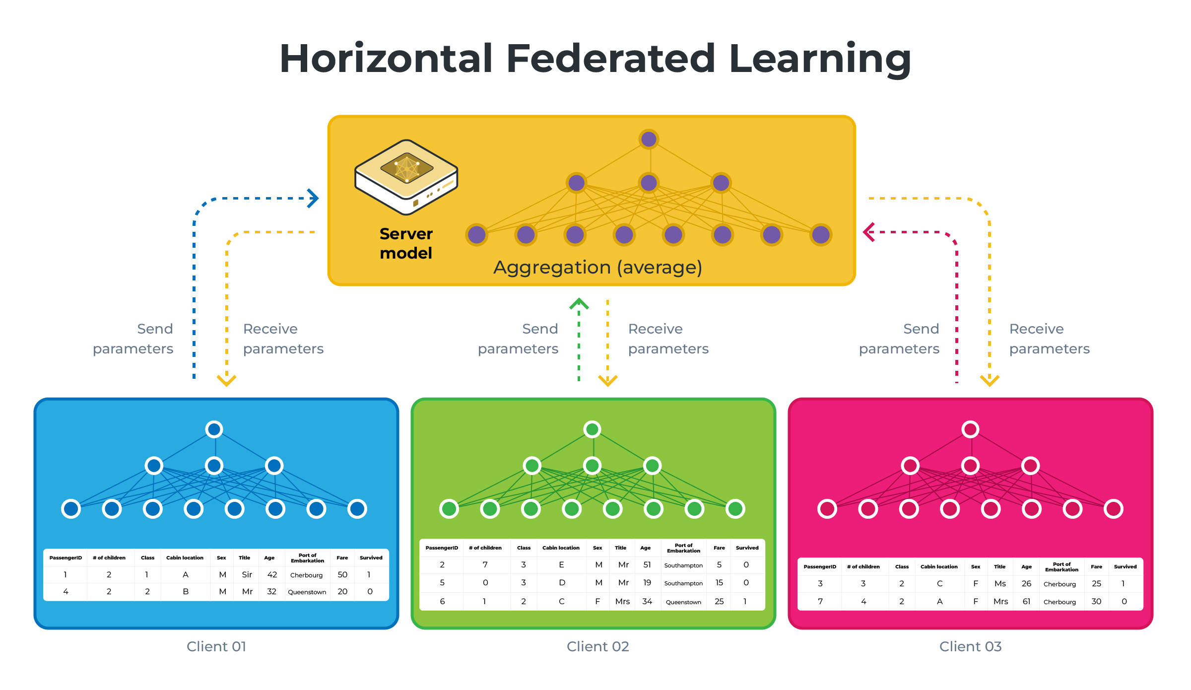
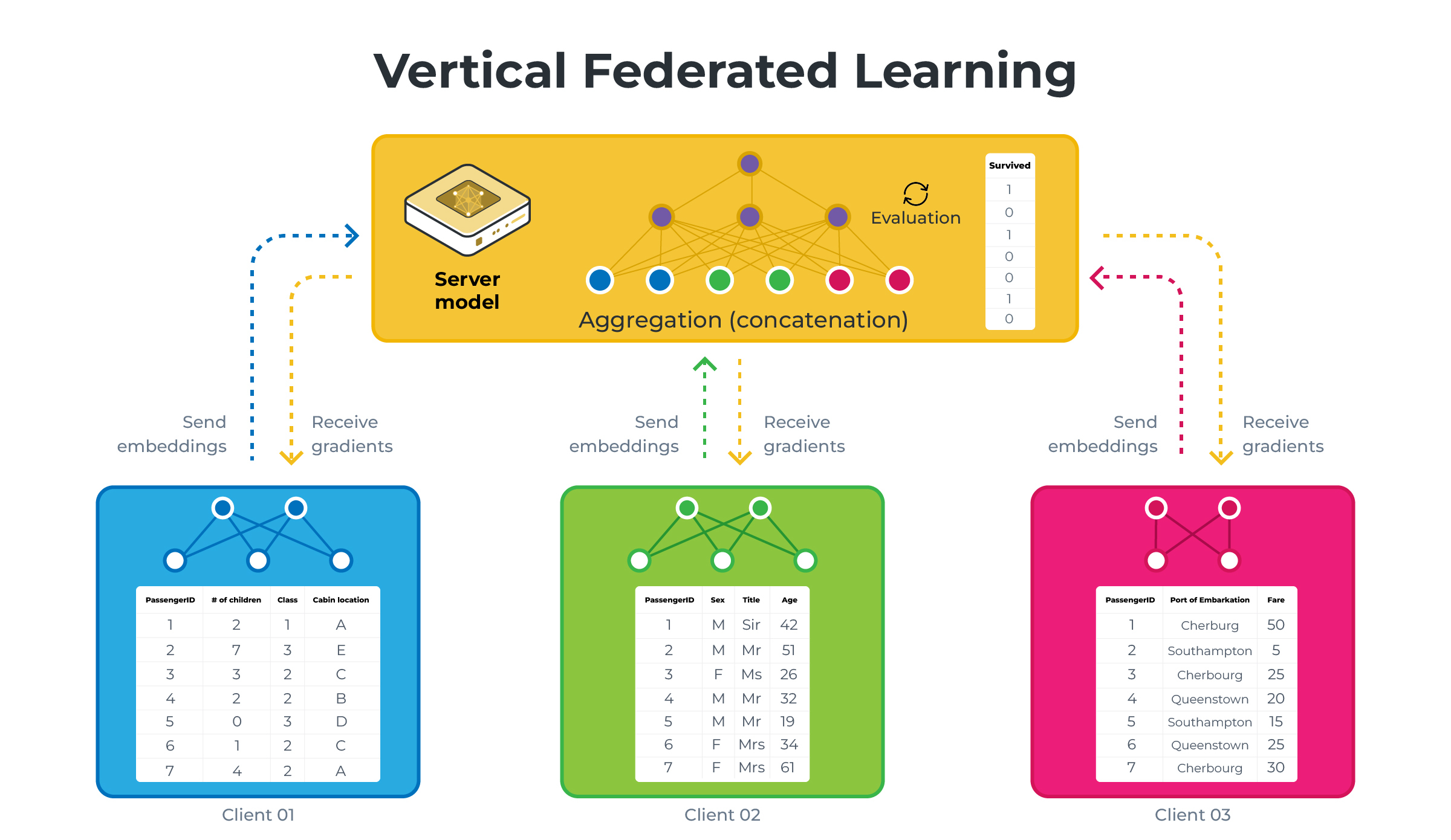
Those diagrams illustrate HFL vs VFL using a simplified version of what we will be building in this example. Note that on the VFL side, the server holds the labels (the Survived column) and computes the training loss and accuracy.

Set up the project¶

Clone the project¶

Start by cloning the example project:

git clone --depth=1 https://github.com/flwrlabs/flower.git _tmp \
        && mv _tmp/examples/vertical-fl . \
        && rm -rf _tmp \
        && cd vertical-fl

This will create a new directory called vertical-fl with the following structure:

vertical-fl
├── vertical_fl
│   ├── __init__.py
│   ├── client_app.py   # Defines your ClientApp
│   ├── server_app.py   # Defines your ServerApp
│   └── task.py         # Defines your model, training and data loading
├── pyproject.toml      # Project metadata like dependencies and configs
└── README.md

Install dependencies and project¶

Install the dependencies defined in pyproject.toml as well as the vertical_fl package.

pip install -e .

Vertical data partitioning¶

In this example we use the VerticalSizePartitioner from Flower Datasets to vertically split the dataset into 3 partitions (one for each client) with the target column (i.e. whether the passenger survived the Titanic sinking) being available at the ServerApp only.

from flwr_datasets import FederatedDataset
from flwr_datasets.partitioner import VerticalSizePartitioner

partitioner = VerticalSizePartitioner(
    partition_sizes=[2, 3, 2], # three partitions with 2,3 and 2 features
    active_party_columns="Survived", # the target
    active_party_columns_mode="create_as_last" # An additional partition will be created 
)                                              # that only contains the target column

fds = FederatedDataset(
    dataset="julien-c/titanic-survival",
    partitioners={"train": partitioner}
)
# Load all partitions
partitions = [fds.load_partition(i) for i in range(fds.partitioners["train"].num_partitions)]

for partition in partitions:
        print(partition.column_names)

# ['Age', 'Sex'] <----------------------------------- ClientApp #0
# ['Fare', 'Siblings/Spouses Aboard', 'Name'] <------ ClientApp #1
# ['Parents/Children Aboard', 'Pclass'] <------------ ClientApp #2
# ['Survived'] <--------------------------------------ServerApp

You can control the number of partitions as well as how many features each have by modifying feature-splits (defaults to [2,3,2]) in the [tool.flwr.app.config] section of the pyproject.toml.

The server reads labels from the final partition of the same FederatedDataset used to load client features. All parties use the same row-shuffle seed, so each embedding row matches its label. This example assumes entities are already aligned. Each process downloads the public dataset before column selection, so the partitioning emulates data ownership rather than enforcing access control.

Each round has two exchanges. The server first collects one embedding block from every feature party, concatenates them in partition order and computes the loss and gradients. It then sends each block’s gradient back to its party and waits for all updates to be acknowledged before starting the next round. Errors or missing feature blocks or acknowledgements abort the run. Each exchange waits up to reply-timeout seconds (120 by default). Increase this setting if a cold dataset download or a slow deployment needs longer.

Run the project¶

You can run your Flower project in both simulation and deployment mode without making changes to the code. If you are starting with Flower, we recommend you using the simulation mode as it requires fewer components to be launched manually. By default, flwr run will make use of the Simulation Engine.

This example is designed to run with three virtual SuperNodes. First we need to change the configuration of the Simulation Runtime (which by default uses 10 nodes). This guide assumes your default SuperLink connection points to one ready for simulations. If you aren’t sure, please refer to the How-to run Flower locally guide.

flwr federation simulation-config --num-supernodes=3

Remember, if you wish to change --num-supernodes you’ll need to adjust feature-splits in the pyproject.toml accordingly.

Run with the Simulation Engine¶

[!NOTE] Check the Simulation Engine documentation to learn more about Flower simulations and how to optimize them.

By default, the example runs for 250 rounds using three clients. Launch it with default settings with:

flwr run .

Training loss and accuracy are logged every 25 rounds and in the final round. Both metrics come from the same forward pass before that round’s model updates. They are measured on the training rows, not a held-out test set, so they do not estimate generalization performance. Results vary with model initialization.

For example, a three-client CPU simulation with the default configuration produced:

INFO :      === Final Results ===
INFO :      Round 25 -> Loss: 0.3622 | Accuracy: 84.55%
INFO :      Round 50 -> Loss: 0.3201 | Accuracy: 87.71%
INFO :      Round 75 -> Loss: 0.2897 | Accuracy: 87.71%
INFO :      Round 100 -> Loss: 0.2638 | Accuracy: 89.18%
INFO :      Round 125 -> Loss: 0.2265 | Accuracy: 90.42%
INFO :      Round 150 -> Loss: 0.2497 | Accuracy: 89.97%
INFO :      Round 175 -> Loss: 0.1962 | Accuracy: 91.43%
INFO :      Round 200 -> Loss: 0.2136 | Accuracy: 91.43%
INFO :      Round 225 -> Loss: 0.1802 | Accuracy: 92.11%
INFO :      Round 250 -> Loss: 0.1484 | Accuracy: 94.25%

You can also override some of the settings for your ClientApp and ServerApp defined in pyproject.toml. For example:

flwr run . --run-config "num-server-rounds=500 learning-rate=0.05"

Run with the Deployment Engine¶

Follow this how-to guide to run the same app in this example but with Flower’s Deployment Engine. After that, you might be intersted in setting up secure TLS-enabled communications and SuperNode authentication in your federation. If you are already familiar with how the Deployment Engine works, you may want to learn how to run it using Docker. Check out the Flower with Docker documentation.